
WAGDA Census Geodatabases
| To facilitate the analysis and mapping of census data, WAGDA has assembled File geodatabases for each of the six counties in Puget Sound Island, King, Kitsap, Pierce, Snohomish, and Thurston, and a geodatabase for Washington State as a whole. Due to changes in the level of detail from the 2000 to 2010 decennial census, the 2010 census does not contain SF3 level survey data. Information about the different survey levels can be found below: SF1 that contains boundary files for mapping at the tract, block group, and block levels and SF3 that contains boundaries for mapping data at the tract and block group levels. The geodatabases can be used with ArcGIS and are stored in ESRI File geodatabase format. |
| Government Publications, Map Collection and Cartographic Information Services, the UW Libraries, or the University of Washington is not responsible for the precision or accuracy of data supplied. All data is provided without warranty. The user of any digital data product accepts it with all faults, and assumes all responsibility for use thereof, and agrees to hold the manufacturer and the University of Washington harmless from and against any damage, loss, or liability arising from any use of the product.
All data within the WAGDA geodatabases is within the public domain. When publishing maps or data from the geodatabase, the U.S. Census Bureau should be cited as the source. |
| 2000 Geodatabase Info | ||
| 1990 Geodatabase Info | ||
The following instructions apply to the 2010 Census geodatabases at the county-level, but the same procedures apply for the state-level database. If you want to use the 1990 or 2010 census geodatabases, you can still follow the general aspects of these instructions, but be sure to read the information on the particular differences between the datasets. The databases are stored in compressed zip files, which can be downloaded and unzipped. These instructions are also available in a text file format on the download page.
Each county-level database has a number of census data tables that contain all of the census data at every geographic level within the county. Each county database also contains two versions of census boundary files at the tract, block group, and block levels one version contains census boundaries that contain water (see Figure 1), while the other is a clipped version that shows only land boundaries (Figure 2). The census boundaries can readily be joined to census data within the database based on a common field, called LOGRECNO. A county boundary, city boundary, and water body features are also included for base-map reference purposes.
|
Figure 1 
This map depicts census boundaries that include land and water. |
Figure 2 
This maps shows census boundaries that have been clipped to include land only. |
Every variable within the database is labeled with a field number. In order to use the data, you must determine the field number that corresponds to the data that you are interested in, and find the table that contains the field number. If you are looking for basic data, like total population, race, age, housing units, etc, you can consult the SF1 or SF3 guide tables for each appropriate year which provide explinations on what each field captures. Simply locate the name of the variable in the list (see Figure 3), and note the table number and field number. Then, within the geodatabase (figure 4), locate the same table, open it, and scroll to the right to find the field (figure 5). Once you have located it, you can add this table to ArcMap to create your map. If you need more detailed census data or you cannot find your variable in the quick reference table, consult either the SF1 Table Matrix or the SF3 Table Matrix, which contains the full list of all variables in the databases.
If you need help with definitions for census bureau variables or geography, consult the American Factfinder Glossary for summary information or download the full SF1 documentation or SF3 documentation from the Census Bureau's website.
|
Figure 3 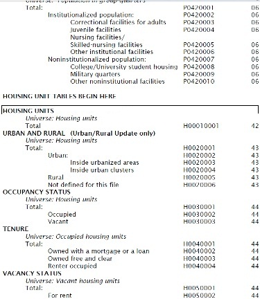 Locate the variable in the reference table, noting the table number and field ID. |
Figure 4 
Open the database (in ArcCatalog) and locate the table. |
|
Figure 5  Open the table and locate the field number. |
Within ArcMap, add the data to the map by going to File > Add data. Once you click on the geodatabase, it will display all of the features and data tables within the database. Select the boundaries and tables that you would like, and add them to the map. Before you can map your data, you must join the data table to your census boundary file based on a common field. To do this, right click on the boundary file in the table of contents and select Joins and Relates > Join (see Figure 6). On the join data screen, choose the LOGRECNO field as the field that you want to base the join on (Figure 7). Then select the appropriate census data table that you wish to join to the layer, and choose the LOGRECNO field as the data table joining field.
|
Figure 6  |
Figure 7  |
Once the tables are joined, you can open the attribute table for the boundary layer, and you will see all of the attribute data for the layer, plus all of the data from the census data table. By opening the properties of the boundary file and selecting the symbology tab, you will be able to map the census data based on quantity by specifying the census data field in the value box (see Figure 8), assuming that you know the field for your variable, based on the reference tables. If you get a message indicating that the maximum sample size has been exceded (this happens if the feature you are mapping contains more than 10,000 records, which frequently happens with census block features), you can increase the sample size by clicking the Classify button, then the Sampling button, and then enter a larger sample size.
|
Figure 8  |
In order to display the features properly, it is best to arrange your layers in the table of contents by keeping the water layer at the bottom and not giving the water any outline, placing the census geography in the middle, and situating the city and county boundaries (if desired) at the top with an outline but no fill (see Figure 9).
|
Figure 9  |
The geodatabases for the State of Washington contain data that can be mapped at the county, census tract, metropolitan area, place (includes incorporated cities and census designated places), and 5-digit ZIP code tabulation areas, in the same manner described above. Please note that the ZIP code boundaries originated from a different source than the other boundaries in the geodatabases. The ZIP boundaries are more generalized, and as such they do not correspond exactly with the other boundary files. For this reason, it is best to use the ZIP boundaries independent of other boundary files. For an explanation of the distinction between ZIP code tabulation areas and USPS ZIP codes, visit the Census Bureau's ZIP Code Tabulation Area (ZCTA) webpage.
Read on for additional instructions (such as how to select census geography for a particular area, like a city, in order to create a new feature that contains only census geography for that city) or go to the download page to download geodatabases, documentation, and metadata. Metadata in a narrative format is also available on the about geodatabases page. There is also a dedicated pages for information about the 1990, 2000 and 2010 census geodatabases.